
Diversifying the customer base is a common tactic companies often take to avoid financial troubles when a central customer experiences unexpected production problems. At the beginning of 2020, México placed 6th worldwide in the manufacturing of light vehicles and 12th in exporting aerospace components. Many companies with a long history in the manufacturing of sheet metal automotive components are preparing diversification plans to include the aerospace industry in their customer portfolios. The aerospace industry is characterized by lightweight components, low volume, and a high combination of part numbers. The main metals used on sheet metal components are aluminum and titanium, which most companies in México lack experience working with.
To help companies with experience only in Low Strength Steels (LSS) or Deep Drawing Steels (DDS) prepare for a possible diversification plan that includes aluminum components, seven critical differences between steel and aluminum are presented below.
- Magnetism
- Young’s modulus
- Deformation capacity after necking
- Lankford coefficient (R-value)
- Strain hardening exponent, n-value
- Slope of extended real strain-stress curve (saturation)
- Deformation capacity on draw operations
Magnetism
Steel presents a Body Centered Cubic (BCC) molecular structure at ambient temperature while aluminum presents Face Centered Cubic (FCC). Anyone can recognize this difference using magnets — steel is strongly attracted by a magnetic force while aluminum is not. This requires several changes to the handling of material, coils, and blanks, and sensing the process inside the press. One example change is the pick and place equipment that uses magnets for steel, which won’t work with aluminum; this would require replacing the robot tips with vacuum systems.
Young’s modulus
This is a mechanical property that measures the tensile stiffness of a solid material. It quantifies the relationship between tensile stress and axial strain in the linear elastic region (see Fig. 1).
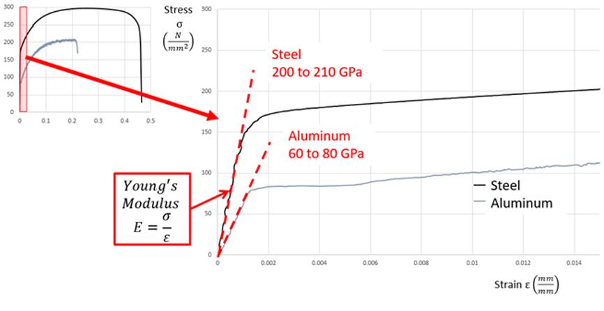
Fig. 1 Difference in the elastic zone in an engineering hardening curve for steel and aluminum
This mechanical property is inversely proportional to the springback results. If two blanks of different materials, one of steel and the other aluminum, are used with the same tooling, the final shape will be different (see Fig. 2). The aluminum component will present higher springback in comparison to the steel component.
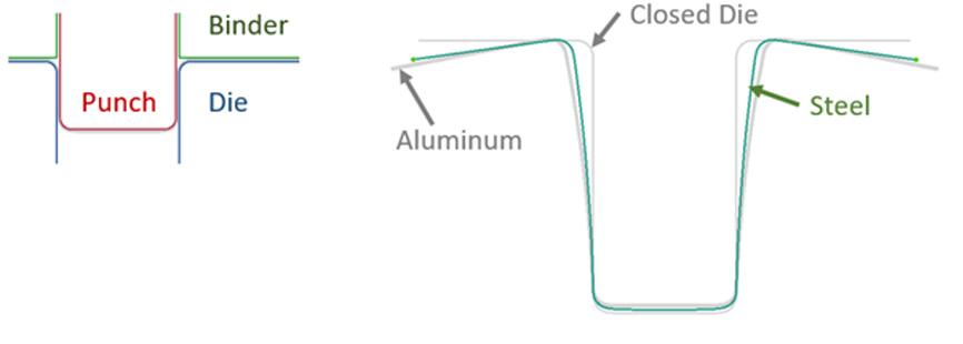
Fig. 2 Comparison of the final shape after drawing between steel and aluminum
Deformation capacity after necking
Nowadays, the onset of necking is considered as failure on draw panels. Necking is presented prior to splits. According to Fig. 3, steel can hold additional deformation after reaching the uniform elongation (UE) limit and the onset of necking, sometimes by almost double the UE limit value. On the other hand, aluminum cannot hold any additional deformation after reaching the UE limit (less than 10% of the UE value).
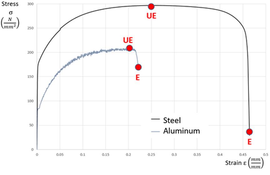
Fig. 3 Comparing elongation (E) and uniform elongation (UE) on engineering strain-stress curves between steel and aluminum
Lankford coefficient (R-value)
The Lankford coefficient, better known as R-value, is the ratio between the strain in the width direction and the reduction in thickness during a tensile test (see Fig. 4). This coefficient can help predict the distribution of superficial and thickness deformation when a material is drawn. As verified in Fig. 5, when the R-value presents a reduced value, the deformation on the surface of the sheet metal is concentrated on the thickness. The same would be true for thickening; when the material is being compressed, under a blankholder for example, materials with a lower R-value will present a significant increase on the thickness during the draw process.
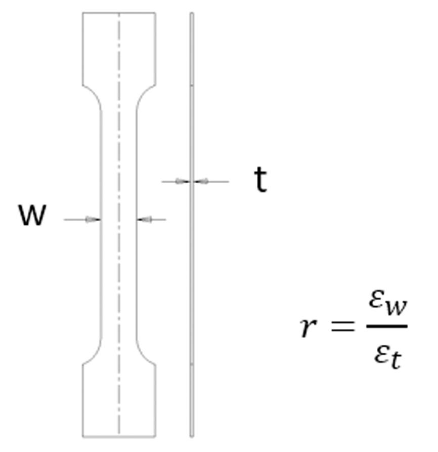
Fig. 4 Equation for the Lankford coefficient (R-value)
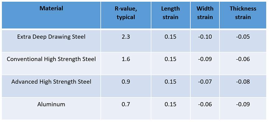
Fig. 5 Distribution of 15% length strain for different materials during tensile test
Strain hardening exponent (n-value)
Modeling the elastic zone in an engineering strain-stress curve is very simple, represented by the line equation using Young’s modulus as the slope. However, representing the plastic zone up to the uniform elongation limit or necking point is more complicated, since the plastic zone is not straight. A common way to model the plastic zone on Deep Drawing Steels is by using the power law equation (Hollomon); see Fig. 6 for a graphical representation of the n-value over the real strain-stress curve. To improve modelling of the plastic zone, the real strain-stress curve is transformed to a logarithmic scale.
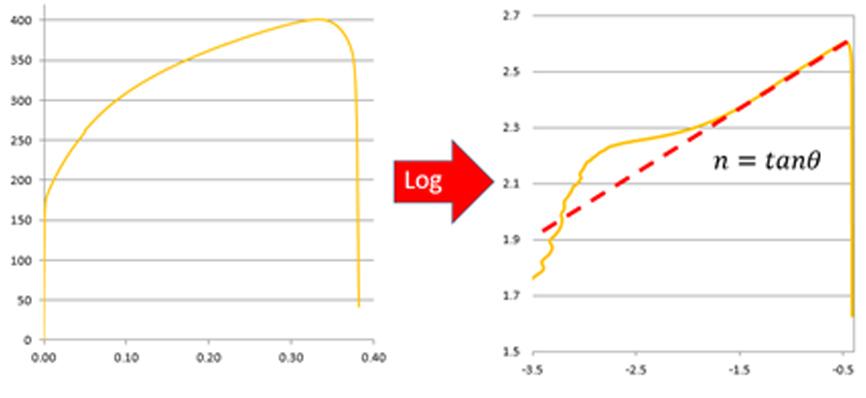
Fig. 6 Graphical representation of the strain hardening exponent (n-value) on a logarithmic scale
The n-value describes how well a material distributes the stress throughout the sheet, thus avoiding the formation of local necks. Fig. 7 presents a comparison between the n-value for DC05 and Aluminum 5754 along plastic deformation until reaching uniform elongation (UE). The n-value for DC05 is considered constant while the n-value for aluminum varies, dropping drastically as the strain reaches UE. This dynamic behavior during the plastic zone reflects that the aluminum will present good capacity to distribute stresses early in the plastic zone, but as the strain increases, the aluminum will tend to present localized necking and split generation.
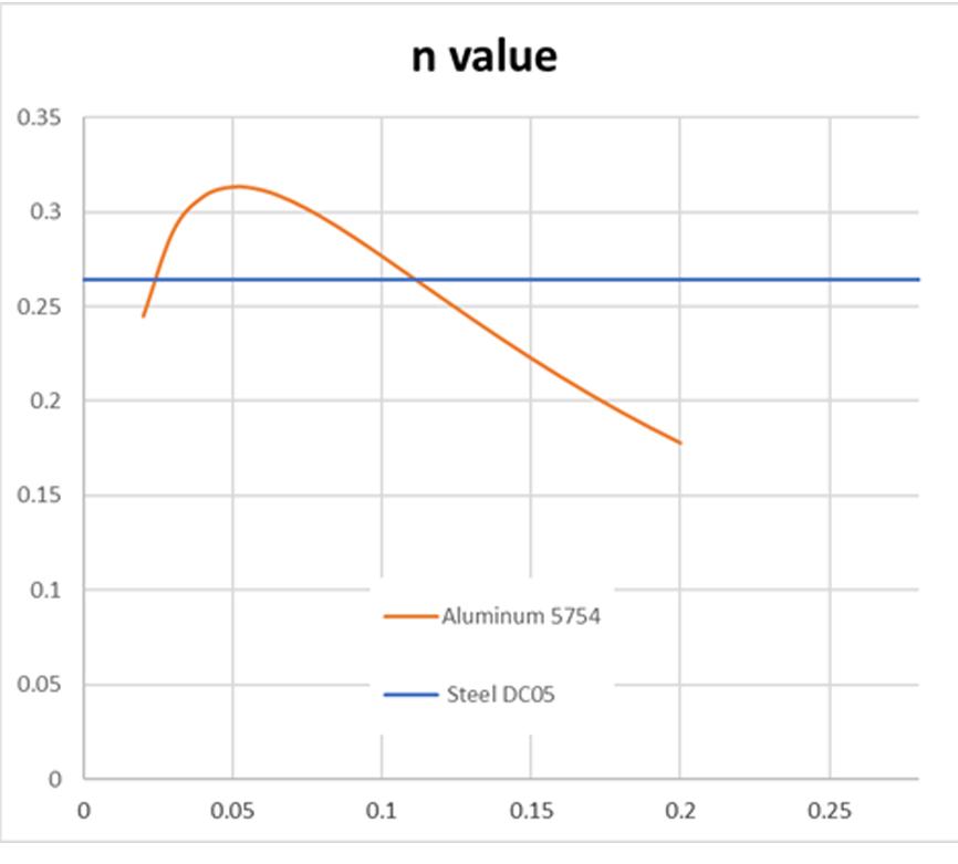
Fig. 7 Comparison of the n-value along plastic deformation until UE for Steel DC05 and Aluminum 5754
Slope of extended real strain-stress curve (saturation)
To facilitate the finite elements calculus, the real strain-stress curve must be extended to 100% deformation. The two extended curves will have different slopes, as shown in Fig. 8. The aluminum slope reduction represents a reduction in its deformation capacity close to and after UE. This means that any increase in stress over the material will cause higher strains, making the tooling tryout more difficult to tune and in some cases, harder to avoid splits.
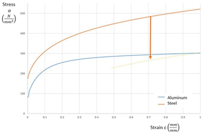
Fig. 8 Comparison of the slope of two real strain-stress curves between steel and aluminum
Deformation capacity on draw operations
The Forming Limit Diagram (FLD) is the most popular criterion for predicting failure in sheet forming operations. It indicates the combination of the major and minor strains that can be applied to a metal sheet without failure. In the ISO 12004 standard, the onset of localized necking is chosen as the sheet failure criterion [1]. Since aluminum presents lower R- and n-values close to UE, the maximum of the forming limit curve (FLC) is smaller compared to DDS, representing a lower strain capacity (see Fig. 9).
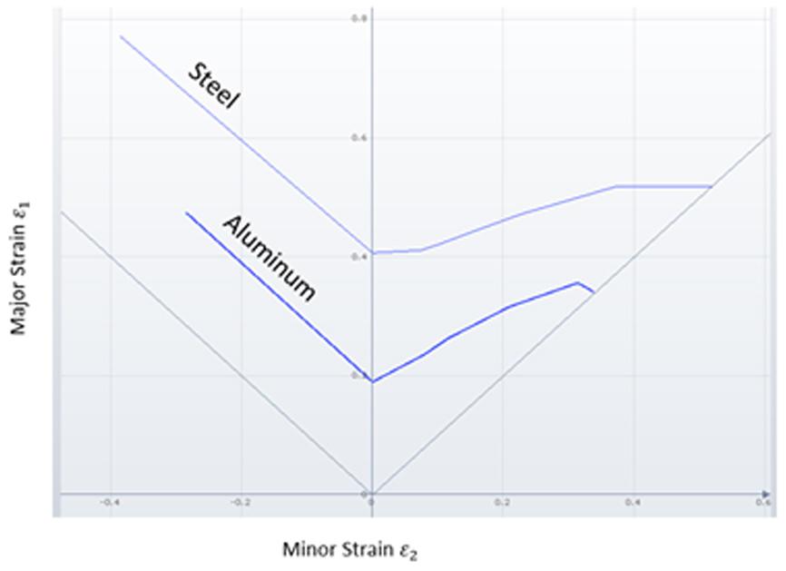
Fig. 9 Comparison of the FLC for aluminum and DDS
[1] S. Bruschi, T. Altan, D. Banabic, P.F. Bariani, A. Brosius, J. Cao, A. Ghiotti, M. Khraisheh, M. Merklein, A.E. Tekkaya (2014) Testing and modelling of material behaviour and formability in sheet metal forming


?")


