
How to get accurate simulations without spending a fortune on complex material testing?
Tata Steel experts have developed advanced material models for forming limit curves and yield loci that are easy to use and improve simulation accuracy without compromising said accuracy. Advanced material models are an important ingredient for improving the accuracy of forming simulations. Unfortunately, these models require input data which is often too time consuming and costly to generate making them impractical for many organisations to use thus restricting their application. At Tata Steel we have recognised this limitation and used our knowledge and expertise to develop different solutions to generating the required input data using minimal testing, without compromising accuracy. In this blog we describe two such solutions: one for accurate yield loci and one for Forming Limit curves (FLC), both generated from simple tensile tests!
The Abspoel & Scholting FLC
The first example is for the Forming Limit Curve. In 2012, Marc Scholting and I developed the Abspoel & Scholting FLC, which calculates the Forming Limit Curve (FLC) from tensile tests using only the total elongation (A80), the strain ratio (r) and the thickness to predict the onset of local necking as depicted in the figure below. Creating an FLC from three tensile test is considerably easier and faster than the traditional method, which in addition requires specialised equipment, operators and lots more material.
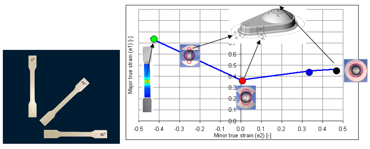
Figure 1: The four points of the Abspoel & Scholting FLC (right) predicted from three directional tensile tests (left shows test samples)
An additional benefit is the ability to generate an FLC in whichever direction you want, relative to the rolling direction, or even all three! You can, for example, choose the direction which has the lowest A80, thus the most critical, rather than sticking to the transverse direction typically done when a measured FLC is made.
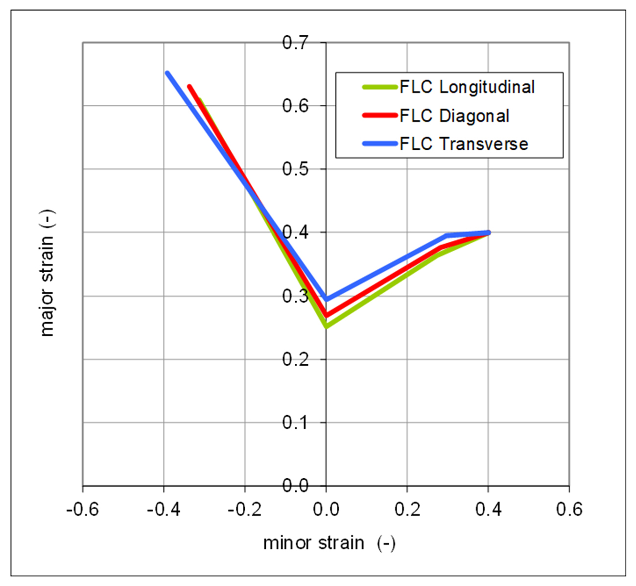
Figure 3: Creation of FLC for different directions
There is a further benefit in the forming process simulation software where the FLC automatically adapts to the initial thickness of the simulated part in the software package. This clearly enables a closer-to-reality scenario compared to one FLC to cover all thicknesses.
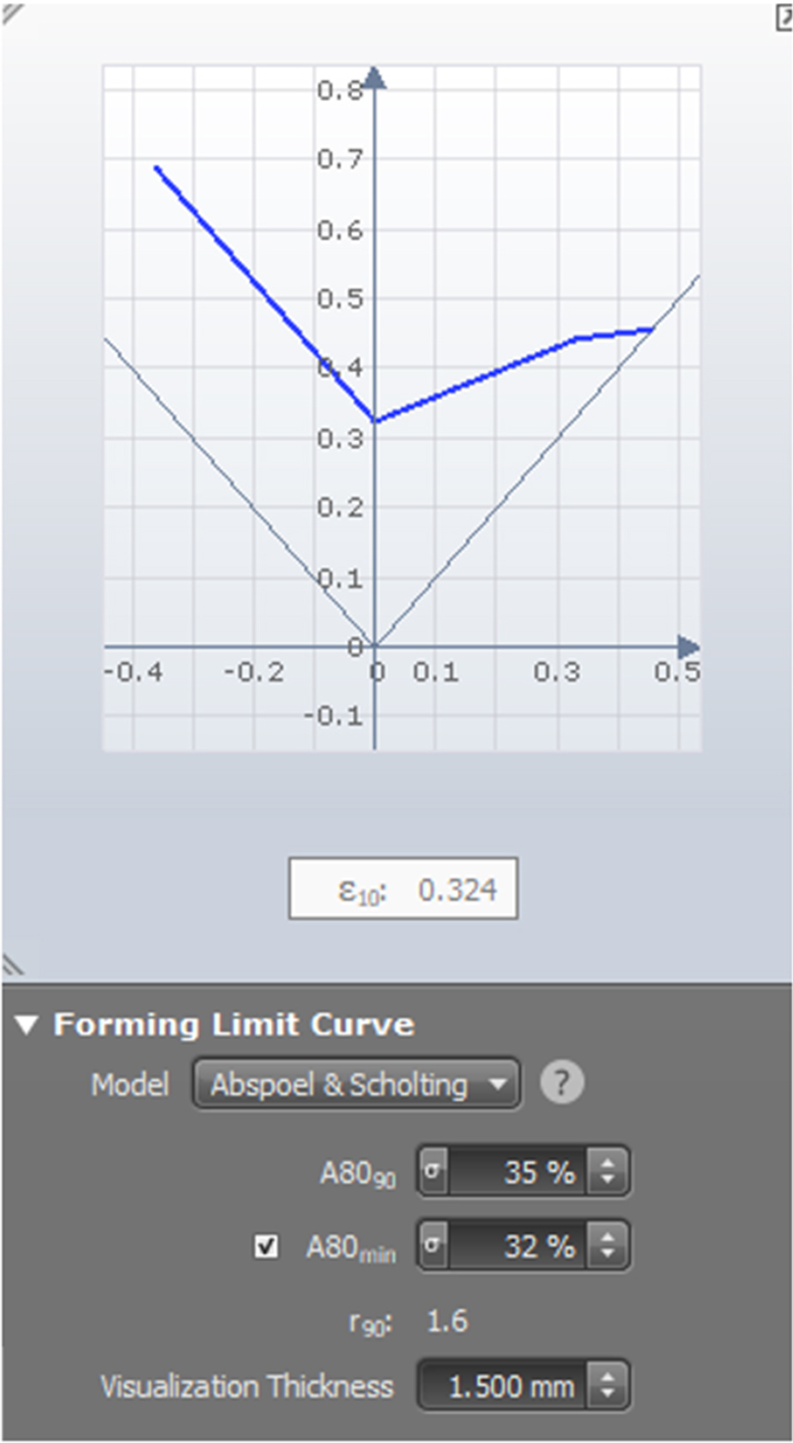
Figure 2: Implementation of the Abspoel & Scholting FLC in AutoForm
Vegter 2017 yield locus
The second example of a time-saving technique is the Tata Steel Vegter 2017 yield locus. The Vegter standard yield locus, which was introduced in 2006, is one of the most accurate due to its interpolating nature. Measured datapoints for uniaxial, plane strain, biaxial and shear stresses are fitted with Bezier curves and therefore use measured data unlike quadratic models. This usage of all measured points was also the drawback of the Vegter standard model because the tests for plane strain and shear are not so easy to perform and not accessible to everybody. Even if you have these tests in-house, it is a huge effort to perform all these special tests for all the materials and their variants.
A huge step forward was made with the development of the Vegter 2017 model. In this, the prediction of shear, plane strain and biaxial stresses are made from only the data of the uniaxial tensile test, similar to the widely used Hill ’48, but maintaining the accuracy of the Vegter standard yield locus. The Vegter 2017 requires 3 directional tensile testing like the Hill’48, but the advanced stress points (shear, plane strain and biaxial) are accurately predicted due to the empirical correlations based on an enormous amount of measured yield loci and corresponding mechanical properties. This is fundamentally different from all the other yield loci which are quadratic equations and have a certain inflexibility.
The equations are publicly available, and peer reviewed by experts of the Journal of Materials Processing Technology. The three directional tensile test results needed are the tensile strength (Rm), the plastic extension at maximum force (or uniform elongation) (Ag), and the plastic strain ratio (r-value).
The yield locus sections for the 0-90 and 45-135 directions are shown in Figure 4. In the Vegter standard model all the points shown on the graph are measured, whereas for the Vegter 2017 only the uniaxial tensile, marked green are measured while the plane strain, shear and biaxial points are all predicted and marked red.
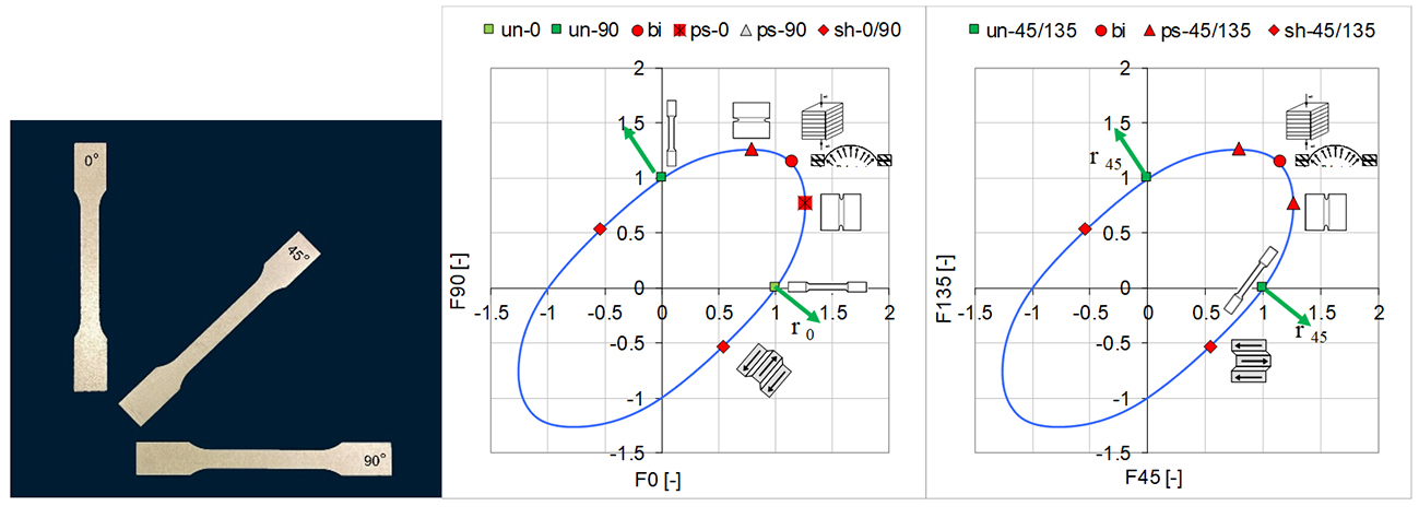
Figure 4: Yield locus for the 0-90 and 45-135 direction.
Using the FLC and yield locus models for simulations
The cooperation of Tata Steel with the FE software suppliers has led to the implementation of both the Abspoel & Scholting FLC and Vegter 2017 in most commonly used forming simulation software (Altair-Radioss, Ansys LS-Dyna, AutoForm, ESI PAM-Stamp, Hexagon MSC Marc, Hexagon Simufact, Stampack Xpress). This widespread implementation makes it possible to use these models globally and interpret the results between different software without material model differences.
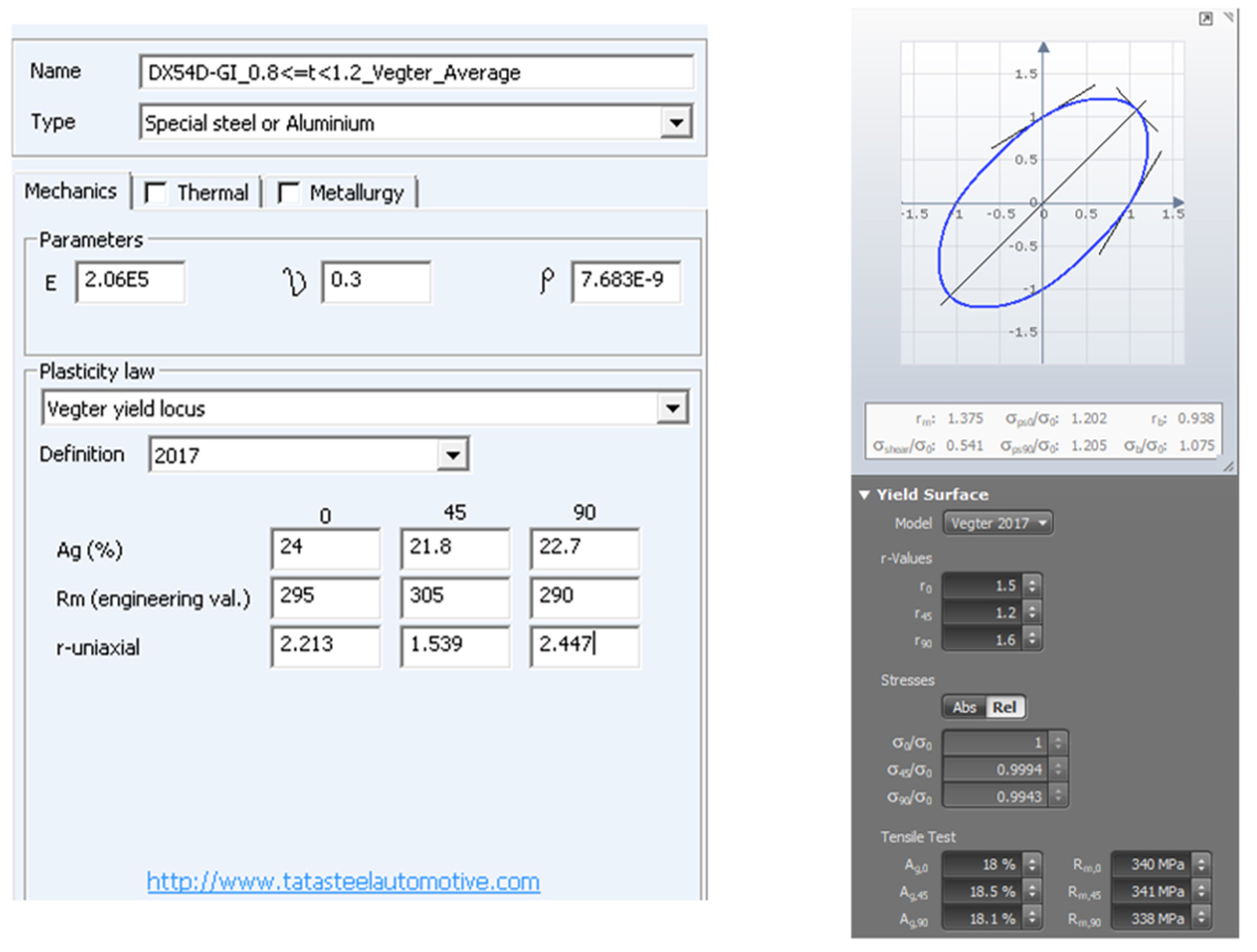
Figure 5: Examples of graphical user interface implementations in FE software.
A simpler way to create accurate advanced material data
To conclude, the ease of use of the Abspoel Scholting FLC model and Vegter 2017 not only makes it simple for every user to create accurate advanced material data, but also enables Tata Steel to create accurate yield loci and FLC’s for all our materials in different thickness ranges.
Tata Steel’s material data is partly available in FE libraries and, more comprehensively, through the Aurora Online service where Tata Steel offers its customers data on the full product range and thickness classes. The data is downloadable as ready to run material decks for the FE codes, as well as datasheets with tabulated data.
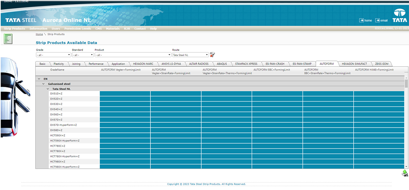
Figure 7: Aurora Online contains different material model combinations per FE code
What’s next? Well, the generated Vegter yield loci for the Tata Steel materials that are available in Aurora® Online are combined with the traditional static hardening curve but also with adiabatic or isothermal hardening curves for different strain rates and temperatures. The latter two are provided to achieve an even higher level of accuracy of the simulation. Strain rate dependent adiabatic hardening curves are recommended for the following reasons:
- More accurate strain prediction in features and critical areas.
- Better force prediction in the part and on the local surfaces (needed for the friction model).
- Adiabatic curves have softening due to heating of the material incorporated. No need to simulate the thermal process during deformation.
- Essential for high-speed forming processes (think of progressive dies or can making).
- Essential for crash simulations.
In the figure below an example for adiabatic hardening curves for different strain rates is shown. In forming processes strain rates up to 10/s are not uncommon on local features. In these areas of the part the strength of the material is higher due to the strain rate response which can result in a change of the strain distribution in the part. As a rule, strain rate dependence mitigates strain localization.
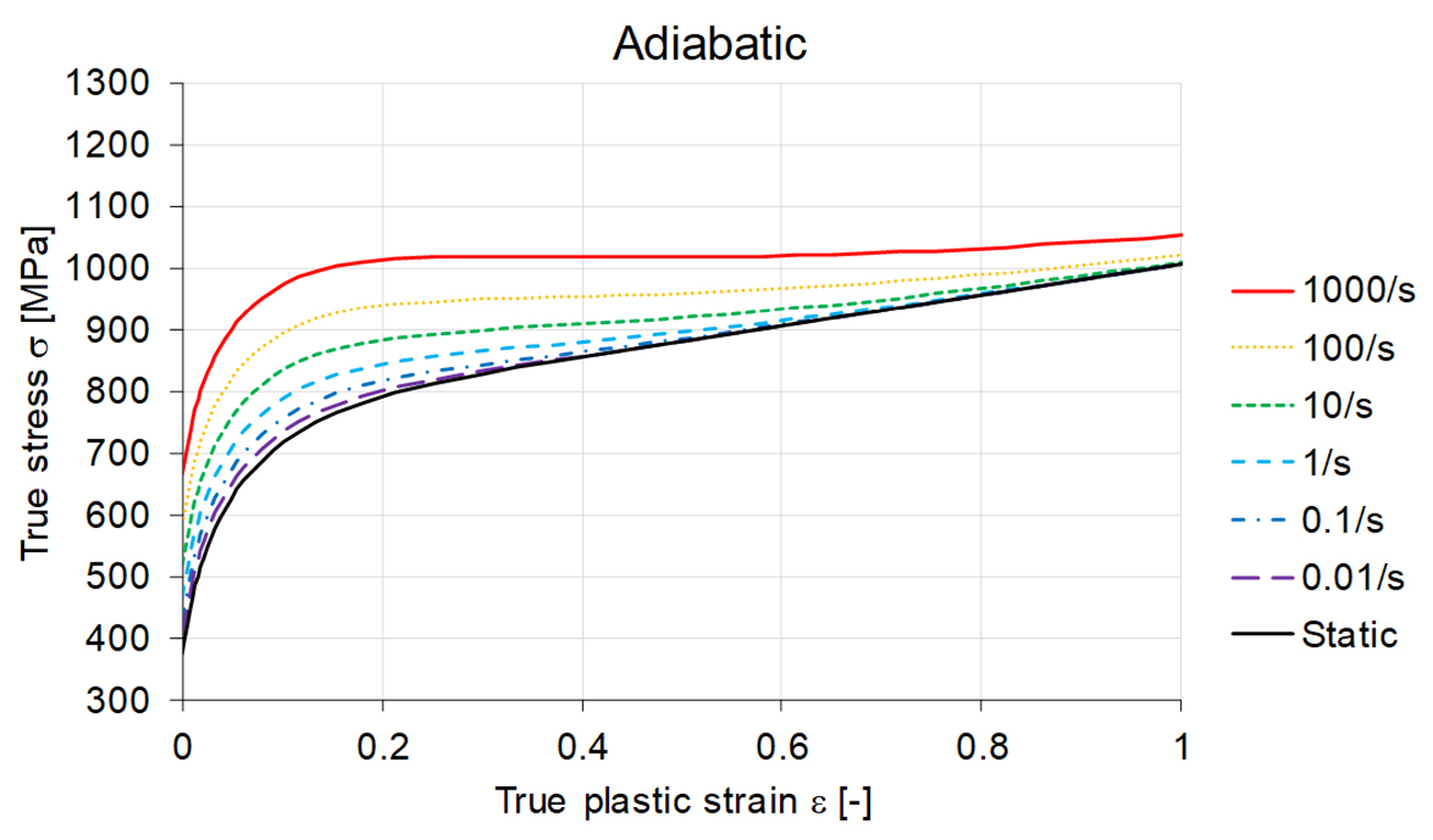
Figure 6: Adiabatic hardening curves for different strain rates
Generating strain rate data can also be an expensive and time consuming activity. Work is ongoing to develop a simplified way to generate this data, thus again enabling the use of the most accurate models with less effort. Further details of this are published on the IDDRG 2019 in the paper thermomechanical forming and crash simulations.
If this article has inspired you to try the Abspoel Scholting FLC model or Vegter 2017 as a practical way to improve simulation accuracy, then you can visit our website and request access to Aurora Online. Our website also has more about Tata Steel knowledge and expertise in material modelling plus a list of published papers


?")


