
Accurately predicting possible failures during the forming process is essential when developing tools. There are many result variables that will offer insight into different failure criteria, including the non-linear FLD, Wrinkles or Surface Lows. In this blog post, AutoForm Technical Product Manager Markus Avermann describes how the FLD evaluates different quality criteria simultaneously.
Every now and then, a customer will ask me whether we still need to use the “old” linear Forming Limit Diagram (FLD) when there are more accurate result variables available.
Well, my answer is that the FLD provides an easily understood overview of many possible failure criteria at once. Although it is not the most accurate way to evaluate a forming process you can quickly find out the critical areas of the part.
Particularly when starting to develop a forming process, you are not interested in the specific details yet, but rather how to adjust e.g. the addendum or the binder shape. After adjusting the tool shape and a new simulation, you can quickly check whether the changes significantly improved the process or made things worse.
Later on, of course, you should use more detailed methods to validate the results. But for initial quick checks, the FLD is the perfect evaluation tool.
So the FLD is still widely used to evaluate a simulation result. But what exactly does it tell us?
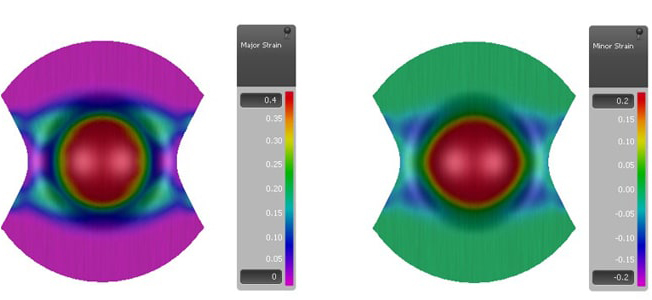
It all starts with the principle strains, i.e. the result variables Major Strain e1 and Minor Strain e2. Here you can switch on either result variable. Then you can consult the distribution on the sheet, represented using different colors.
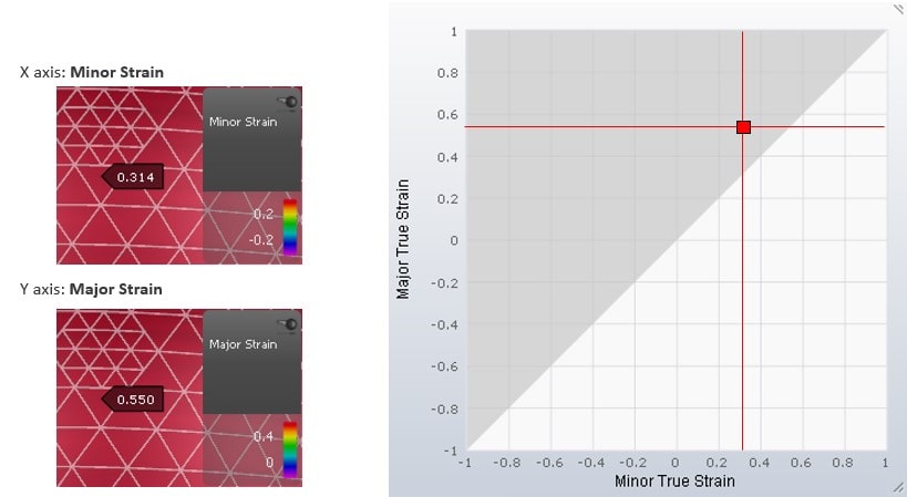
But you can gather even more information if you look at both variables at once. This is possible if you transfer the results of a simulated element into a diagram. In this diagram, the Y-axis represents the Major Strain values and the X-axis represents the Minor Strain values. If we mark both principle strains in the diagram, it is called the strain state of an element.
The Major Strain is always defined as the higher principle strain and the Minor Strain is defined as the lower principle strain. Therefore, we will see only strain states in the grey area of the diagram.
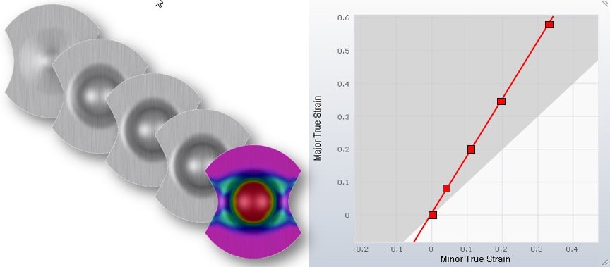
If we put the strains of different time steps into the diagram, we can connect the strain states with a curve. This curve is called the strain path. In some forming processes, the ratio between the Major Strain and the Minor strain is always the same. In this case, when marking the strain states on the diagram, and connecting them, the resulting curve is a straight line. This is called a linear strain path.
A real sheet will at some point crack during forming. This can also be visualized in the diagram. There are material tests, e.g. the Nakajima test, that have been developed specifically to represent the cracking behavior of sheet metal.
The resulting strain state in the center of the specimen depends on its shape. In addition, the strain path is linear. Now tests are performed until the specimen experiences necking. The principle strains are measured continuously throughout the test. So in the end, we know the strain state when the necking begins.
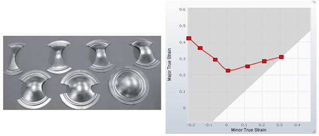
When running several material tests with differently shaped specimens, we get differing strain states that lead to necking of the sheet.
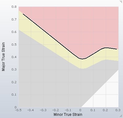
We can put these necking strain states into the diagram and connect them with a curve. This curve represents the limit of forming without cracks. It is called the Forming Limit Curve (FLC).
For a clearer understanding, we can change the background colors in the diagram. The area above the FLC has been changed to red. So any strain state in the red area indicates a failure due to necking. In addition, there is a yellow area immediately below the FLC to warn you that a strain state is close to failure.
So far, we have only considered the Major Strain and Minor Strain. These are the strains in the plane of the sheet. But of course, there is also a strain in the thickness direction. This strain is usually represented by the result variable Thinning.
Keep in mind that the result variable Thinning shows an engineering strain, whereas Major Strain and Minor Strain are true strains.
One of the basic boundary conditions of a simulation result is that the volume of the sheet does not change due to its plastic incompressibility. In other words, regardless of how the sheet is formed, the sum of the principle strains (true strain) in all 3 directions is always as follows:
![]()
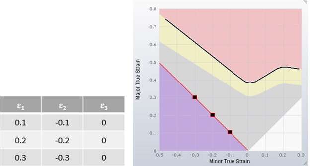
If we examine strain states where the strain in the thickness direction is 0, it turns out that the Minor Strain is just the negative value of the Major Strain. When inputting some possible strain states into the diagram, the connecting line forms a 45° angle. Along this line, the thinning is exactly 0. Any strain state to the left of this line represents thickening, while any strain state to the right of this line represents thinning. Any strain state involving thickening can be identified when adding a purple area to the diagram.
When checking the quality of a formed part, there are additional limits of Thinning to be considered. The limit of Thinning is often 25% or 30%. There may be a minimum part thickness required to fulfill the function of the part, or a high Thinning may lead to a bad surface texture of certain materials.
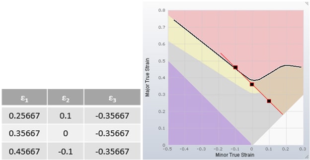
These limits can also be represented in the diagram. Let’s assume the limit of Thinning is 30%. The corresponding value of the result variable Thinning in AutoForm is an engineering strain of -0.3. As mentioned before, we have to transform this engineering strain into a true strain before calculating strain states for the diagram.
![]()
Now we can add a few strain states into the diagram that represent a thinning of 30% and we can connect these strain states. Again, this area of the diagram has a boundary line forming a 45° angle. Any strain state to the right of this line represents a thinning higher than 30%. This area is indicated in orange.
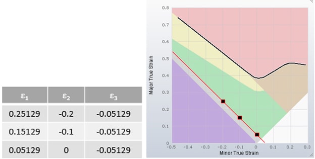
Another intersting thinning value might be 3% or 5%. These values are considered to check whether the sheet is stretched well enough to reduce springback and a tendency towards surface defects. This can also be visualized in the diagram. First, we have to transform the 5% thinning into a true strain.
![]()
Adding reference strain states to the diagram results in an additional area, which is represented in green. Strain states in the green area are assumed to indicate a well stretched sheet.
Finally there are strain states that refer to the uniaxial stress state, e.g. the tensile test. For this use case, the ratio of Major to Minor Strain depends on the average r-value of the material.
ε1= -(ε2 + ε2/rm)
If we input strain states that correspond to uniaxial stress, we can define another region in the diagram. Any strain state on the right of the uniaxial stress line has a more or less biaxial stress. Whereas any strain state on the left of the uniaxial stress line has a component of compressive stress.
This additional area is indicated in blue. Since compressive stress can lead to wrinkles, the blue area represents a risk of wrinkles.
In AutoForm, you can visualize the strain states of all the elements in the Forming Limit Diagram (FLD). In addition, we use the colors from the FLD to indicate the corresponding strain state of the sheet elements. This result variable is called Formability.
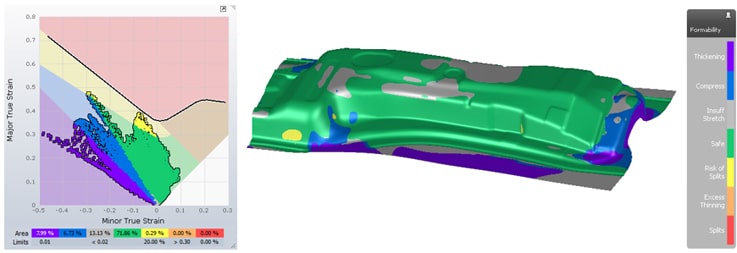
Although there are result variables that offer more detailed information about a single quality criterion, the FLD provides a good overview. Particularly for early feasibility studies, Formability helps to quickly identify critical areas that require further investigation.


